 4 第四章 习题 参考答案.docx
- 文档编号:14513877
- 上传时间:2023-06-24
- 格式:DOCX
- 页数:20
- 大小:111.67KB
4 第四章 习题 参考答案.docx
《4 第四章 习题 参考答案.docx》由会员分享,可在线阅读,更多相关《4 第四章 习题 参考答案.docx(20页珍藏版)》请在冰点文库上搜索。
4第四章习题参考答案
第四章习题参考答案P135
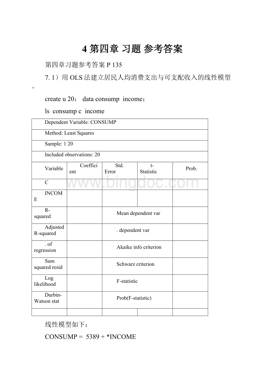
7.1)用OLS法建立居民人均消费支出与可支配收入的线性模型。
createu20;dataconsumpincome;
lsconsumpcincome
DependentVariable:
CONSUMP
Method:
LeastSquares
Sample:
120
Includedobservations:
20
Variable
Coefficient
Std.Error
t-Statistic
Prob.
C
INCOME
R-squared
Meandependentvar
AdjustedR-squared
.dependentvar
.ofregression
Akaikeinfocriterion
Sumsquaredresid
Schwarzcriterion
Loglikelihood
F-statistic
Durbin-Watsonstat
Prob(F-statistic)
线性模型如下:
CONSUMP=5389+*INCOME
2)检验模型是否存在异方差性
i)
图:
是否有明显的散点扩大/缩小/复杂型趋势
scatincomeconsump
ii)解释变量—残差图:
是否形成一条斜率为0的直线
scatincomeresid^2或者
genrei2=resid^2;scatincomeei2
由两个图形,均可判定存在递增型异方差。
还可以用帕克检验,戈里瑟检验,戈德菲尔德-匡特检验,怀特检验等方法。
iii)戈德菲尔德-匡特检验:
共有20个样本,去掉中间1/4个样本(4个),剩余大样本、小样本各8个。
Sortincome;smpl18;lsconsumpCincome
Smpl1320;lsconsumpCincome
,存在异方差。
iV)怀特检验:
因为只有一个变量,故是否含有交叉项是一样的。
View\residualtest\whiteheteroskedastcity
(crossterms/nocrossterms)
WhiteHeteroskedasticityTest:
F-statistic
Probability
Obs*R-squared
Probability
DependentVariable:
RESID^2
Method:
LeastSquares
Sample:
120
Includedobservations:
20
Variable
Coefficient
Std.Error
t-Statistic
Prob.
C
INCOME
INCOME^2
R-squared
Meandependentvar
AdjustedR-squared
.dependentvar
.ofregression
Akaikeinfocriterion
Sumsquaredresid
+10
Schwarzcriterion
Loglikelihood
F-statistic
Durbin-Watsonstat
Prob(F-statistic)
,存在异方差。
还可以通过概率
判定存在异方差。
3)若存在异方差,用适当的方法估计模型对数(加权最小二乘法)
lsconsumpCincome;genreijdz=abs(resid)
ls(w=1/eijdz)consumpCincome
DependentVariable:
CONSUMP
Method:
LeastSquares
Sample:
120
Includedobservations:
20
Weightingseries:
1/EIJDZ
Variable
Coefficient
Std.Error
t-Statistic
Prob.
C
INCOME
WeightedStatistics
R-squared
Meandependentvar
AdjustedR-squared
.dependentvar
.ofregression
Akaikeinfocriterion
Sumsquaredresid
Schwarzcriterion
Loglikelihood
F-statistic
Durbin-Watsonstat
Prob(F-statistic)
UnweightedStatistics
R-squared
Meandependentvar
AdjustedR-squared
.dependentvar
.ofregression
Sumsquaredresid
Durbin-Watsonstat
WhiteHeteroskedasticityTest:
F-statistic
Probability
Obs*R-squared
Probability
TestEquation:
DependentVariable:
STD_RESID^2
Method:
LeastSquares
Sample:
120
Includedobservations:
20
Variable
Coefficient
Std.Error
t-Statistic
Prob.
C
INCOME
或
均可判定加权处理后的模型不存在异方差。
模型经取对数或加权处理都可以一定程度地消除异方差性。
lslog(consump)Clog(income);genreijdz=abs(resid);
ls(w=1/eijdz)log(Consump)Clog(Income)
普通最小二乘模型
CONSUMP=5389+*INCOME
加权最小二乘模型
CONSUMP=+*INCOME
对数模型:
LOG(CONSUMP)=+*LOG(INCOME)
加权对数模型:
LOG(CONSUMP)=+*LOG(INCOME)
对各种模型的White检验结果,综合如下
模型不取对数
F-statistic
Probability
Obs*R-squared
Probability
模型取对数
F-statistic
Probability
Obs*R-squared
Probability
模型不取对数,但加权
F-statistic
Probability
Obs*R-squared
Probability
模型取对数,且加权
F-statistic
Probability
Obs*R-squared
Probability
可见,各种方法都可以起到抑制异方差的效果。
8.1)若采用对数模型,是否存在序列相关性
lslog(industry)Clog(invest)
DependentVariable:
LOG(INDUSTRY)
Method:
LeastSquares
Sample:
19011921
Includedobservations:
21
Variable
Coefficient
Std.Error
t-Statistic
Prob.
C
LOG(INVEST)
R-squared
Meandependentvar
AdjustedR-squared
.dependentvar
.ofregression
Akaikeinfocriterion
Sumsquaredresid
Schwarzcriterion
Loglikelihood
F-statistic
Durbin-Watsonstat
Prob(F-statistic)
LOG(INDUSTRY)=1.+*LOG(INVEST)
i)
散点图
ii)
随t变化的散点图
由两个图形,均可判定存在正序列相关。
还可以利用回归检验法,D-W检验,拉格朗日乘数检验等方法。
iii)D-W检验(DL(21,=,DU(21,=
.= iv)拉格朗日乘数检验 Breusch-GodfreySerialCorrelationLMTest: F-statistic Probability Obs*R-squared Probability Variable Coefficient Std.Error t-Statistic Prob. C LOG(INVEST) RESID(-1) R-squared Meandependentvar AdjustedR-squared .dependentvar Loglikelihood F-statistic Durbin-Watsonstat Prob(F-statistic) 一阶LMTest: LMTest RESID(-1)的t统计量显著(P=<),至少存在一阶自相关。 2)按照一阶自相关,用杜宾两步法和广义最小二乘法估计原模型。 杜宾两步法: lsycy(-1)xx(-1) y(-1)前面的系数: ,代回差分模型 ,再次进行OLS估计得到原模型的参数估计量,即 。 genry=log(industry);genrx=log(invest); Step1: lsycy(-1)xx(-1) DependentVariable: Y Method: LeastSquares Sample(adjusted): 19812000 Includedobservations: 20afteradjustingendpoints Variable Coefficient Std.Error t-Statistic Prob. C Y(-1) X X(-1) R-squared Meandependentvar AdjustedR-squared .dependentvar .ofregression Akaikeinfocriterion Sumsquaredresid Schwarzcriterion Loglikelihood F-statistic Durbin-Watsonstat Prob(F-statistic) Step2: lsy-*y(-1)cx-*x(-1) DependentVariable: *Y(-1) Method: LeastSquares Sample(adjusted): 19812000 Includedobservations: 20afteradjustingendpoints Variable Coefficient Std.Error t-Statistic Prob. C *X(-1) R-squared Meandependentvar AdjustedR-squared .dependentvar .ofregression Akaikeinfocriterion Sumsquaredresid Schwarzcriterion Loglikelihood F-statistic Durbin-Watsonstat Prob(F-statistic) .=介于DL(21-1,2,=与DU(21-1,2,=之间,不能判别是否存在一阶正自相关,但可由拉格朗日乘数法判断,此时不存在序列相关性。 Breusch-GodfreySerialCorrelationLMTest: F-statistic Probability Obs*R-squared Probability TestEquation: DependentVariable: RESID Method: LeastSquares Variable Coefficient Std.Error t-Statistic Prob. C *X(-1) RESID(-1) R-squared Meandependentvar AdjustedR-squared .dependentvar .ofregression Akaikeinfocriterion Sumsquaredresid Schwarzcriterion Loglikelihood F-statistic Durbin-Watsonstat Prob(F-statistic) 拉格朗日乘数检验: D-Wstat: >,不存在序列相关性。 所以 矫正后的模型: LOG(INDUSTRY)=+*LOG(INVEST) 原模型: LOG(INDUSTRY)=1.+*LOG(INVEST) 广义差分法 lsycxar (1) (不能判定是否存在一阶自相关) DependentVariable: Y Method: LeastSquares Sample(adjusted): 19812000 Includedobservations: 20afteradjustingendpoints Convergenceachievedafter15iterations Variable Coefficient Std.Error t-Statistic Prob. C X AR (1) R-squared Meandependentvar AdjustedR-squared .dependentvar .ofregression Akaikeinfocriterion Sumsquaredresid Schwarzcriterion Loglikelihood F-statistic Durbin-Watsonstat Prob(F-statistic) 但由LM检验: 概率为>,故此时不存在序列相关性。 因此模型只存在一阶自相关性。 Breusch-GodfreySerialCorrelationLMTest: F-statistic Probability Obs*R-squared Probability DependentVariable: RESID Variable Coefficient Std.Error t-Statistic Prob. C X AR (1) RESID(-1) Durbin-Watsonstat Prob(F-statistic) 模型为Y=+*X+*AR (1)与杜宾两步法矫正的模型: LOG(INDUSTRY)=+*LOG(INVEST)非常接近。 广义最小二乘法 若仅存在一阶自相关 lslog(industry)Clog(invest)genrresid_corr=resid lsresid_corrCresid_corr(-1)注: resid是内置变量; DependentVariable: RESID_CORR Method: LeastSquares Variable Coefficient Std.Error t-Statistic Prob. C RESID_CORR(-1) R-squared Meandependentvar Durbin-Watsonstat Prob(F-statistic) 直接计算 模型为LOG(INDUSTRY)=+*LOG(INVEST),误差偏大。 3)采用差分形式 ,估计原模型 。 lsD(industry)CD(invest) OR COMMAND lsindustry–industry(-1)Cinvest–invest(-1) DependentVariable: D(INDUSTRY) Method: LeastSquares Sample(adjusted): 19812000 Includedobservations: 20afteradjustingendpoints Variable Coefficient Std.Error t-Statistic Prob. C D(INVEST) R-squared Meandependentvar AdjustedR-squared .dependentvar .ofregression Akaikeinfocriterion Sumsquaredresid Schwarzcriterion Loglikelihood F-statistic Durbin-Watsonstat Prob(F-statistic) Breusch-GodfreySerialCorrelationLMTest: F-statistic Probability Obs*R-squared Probability TestEquation: DependentVariable: RESID Method: LeastSquares Variable Coefficient Std.Error t-Statistic Prob. C D(INVEST) RESID(-1) R-squared Meandependentvar AdjustedR-squared .dependentvar .ofregression Akaikeinfocriterion Sumsquaredresid Schwarzcriterion Loglikelihood F-statistic Durbin-Watsonstat Prob(F-statistic) 原模型存在一阶正自相关,但经过一阶自相关差分处理后不存在序列相关性(.=>或P=>)。 模型为: D(INDUSTRY)=+*D(INVEST) 说明: 在有的方法不能判别自相关性时,可以用其他方法测试。 9.说明下述回归模型是否可靠 LsCONSUMPCINCOMEWEALTH DependentVariable: CONSUMP Method: LeastSquares Sample: 110 Includedobservations: 10 Variable Coefficient Std.Error t-Statistic Prob. C INCOME WEALTH R-squared Meandependentvar AdjustedR-squared .dependentvar .ofregression Akaikeinfocriterion Sumsquaredresid Schwarzcriterion Loglikelihood F-statistic Durbin-Watsonstat Prob(F-statistic) DependentVariable: CONSUMP Variable Coefficient Std.Error t-Statistic Prob. INCOME C DependentVariable: CONSUMP Variable Coefficient Std.Error t-Statistic Prob. WEALTH C DependentVariable: INCOME Variable Coefficient Std.Error t-Statistic Prob. WEALTH C R-squared Meandependentvar AdjustedR-squared .dependentvar .ofregress


- 配套讲稿:
如PPT文件的首页显示word图标,表示该PPT已包含配套word讲稿。双击word图标可打开word文档。
- 特殊限制:
部分文档作品中含有的国旗、国徽等图片,仅作为作品整体效果示例展示,禁止商用。设计者仅对作品中独创性部分享有著作权。
- 关 键 词:
- 第四章 习题 参考答案 第四
 冰点文库所有资源均是用户自行上传分享,仅供网友学习交流,未经上传用户书面授权,请勿作他用。
 《畜牧学概论》复习题.docx
-
《工贸行业较大危险因素辨识与防范指导手册版》使用指南.docx
-
《家电延保计划书》.docx
-
《木材学》试 卷 答 案.docx
-
《田家四季歌》教学反思.docx
-
《修优美师德做阳光教师》读书笔记700字5篇最新范文.docx
-
0江南逢李龟年诗歌板书设计.docx
-
3套打包沧州六年级下册英语期中单元检测试题解析版.docx
-
13年助理医师模拟题病理学27页word资料.docx
-
037全国自考美学历年真题及答案.docx
-
310北京研讨会数学.docx
-
ABCD 世界四大粮商的前世今生.docx
-
《初级会计实务》笔记与真题.docx
-
《工程荷载与可靠度设计原理》课后思考题及复习详解1解析.docx
-
《计算机硬件组装与维护》教案.docx
-
《面向对象分析与设计UML》期末总复习.docx
-
《天津市土地管理条例》.docx
-
《信息安全等级保护测评机构管理办法》最新.docx
-
《左传》翻译练习及参考答案.docx
-
3手术衣医疗器械安全有效基本要求清单0821.docx
-
12压力容器压力管道设计许可规则.docx
-
《白洋淀纪事》教案知识讲解.docx
-
《耳朵上的绿星》教案.docx
-
《会计学基础》考试试题及答案.docx
-
《白鹅》教学设计范文通用9篇.docx
-
《流浪地球》观后感15篇.docx
-
《东北地区》练习题.docx
-
《皇帝的新衣》读后感.docx
-
《伶官传序》讲解及知识训练.docx
-
《市场营销学》形考答案.docx
-
《小池》教学反思.docx
-
《别踩白块度典范版》设计计划文档.docx
-
武汉市购房合同范本3篇.docx
-
推荐三年级上册英语教案Unit 4 We love animals We love animals 人教PEPdoc.docx
-
外贸信函查询.docx
-
五百次的回眸.docx
-
小学英语教师述职报告范文五篇.docx
-
五年级英语下册unit 4 when is easter教案.docx
-
外科护理学试题500题.docx
-
物联网产业发展与人才需求调研报告最终版讲解共10页.docx
-
五一劳动节宣传栏.docx
-
外贸业务员实习周记500字.docx
-
小篆.docx
-
外圆磨床岗位作业指导书.docx
-
校友会发言稿.docx
-
外墙岩棉板保温施工综合方案样本.docx
-
外研版学年三年级英语三起下学期全册教案.docx
-
写话训练段落2.docx
-
完整版ncl函数大全.docx
-
完美升级版G312线至西山乡公路改建工程项目施工设计文字说明.docx
-
西城区中考二模语文试题及答案.docx
