 数值分析作业MATLAB.docx
- 文档编号:15517080
- 上传时间:2023-07-05
- 格式:DOCX
- 页数:12
- 大小:17.75KB
数值分析作业MATLAB.docx
《数值分析作业MATLAB.docx》由会员分享,可在线阅读,更多相关《数值分析作业MATLAB.docx(12页珍藏版)》请在冰点文库上搜索。
数值分析作业MATLAB
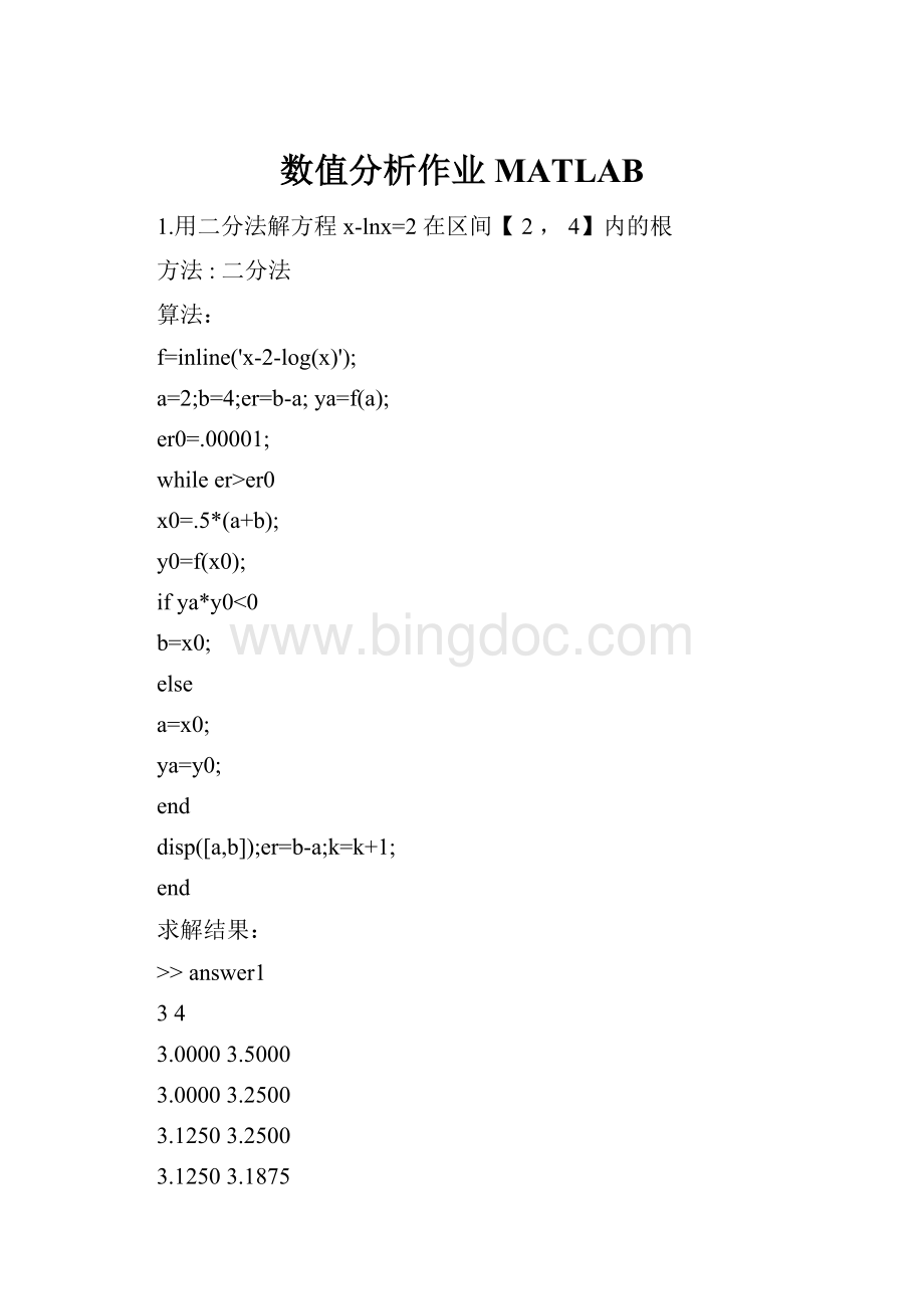
1.用二分法解方程x-lnx=2在区间【2,4】内的根
方法:
二分法
算法:
f=inline('x-2-log(x)');
a=2;b=4;er=b-a;ya=f(a);
er0=.00001;
whileer>er0
x0=.5*(a+b);
y0=f(x0);
ifya*y0<0
b=x0;
else
a=x0;
ya=y0;
end
disp([a,b]);er=b-a;k=k+1;
end
求解结果:
>>answer1
34
3.00003.5000
3.00003.2500
3.12503.2500
3.12503.1875
3.12503.1563
3.14063.1563
3.14063.1484
3.14453.1484
3.14453.1465
3.14553.1465
3.14603.1465
3.14603.1462
3.14613.1462
3.14623.1462
3.14623.1462
3.14623.1462
3.14623.1462
最终结果为:
3.1462
2.试编写MATLAB函数实现Newton插值,要求能输出插值多项式。
对函数
1
f(x)21在区间[-5,5]上实现10次多项式插值。
4x1
Matlab程序代码如下:
%此函数实现y=1/(1+4*x^2)的n次Newton插值,n由调用函数时指定
%函数输出为插值结果的系数向量(行向量)和插值多项式
算法:
function[ty]=func5(n)
x0=linspace(-5,5,n+1)';
y0=1./(1.+4.*x0.^2);
b=zeros(1,n+1);
fori=1:
n+1
s=0;
forj=1:
i
t=1;
fork=1:
i
ifk~=j
t=(x0(j)-x0(k))*t;
end;
end;
s=s+y0(j)/t;
end;
b(i)=s;
end;
t=linspace(0,0,n+1);
fori=1:
n
s=linspace(0,0,n+1);
s(n+1-i:
n+1)=b(i+1).*poly(x0(1:
i));
t=t+s;
end;
t(n+1)=t(n+1)+b
(1);
y=poly2sym(t);
10次插值运行结果:
[bY]=func5(10)
b=
Columns1through4
-0.00000.00000.0027-0.0000
Columns5through8
-0.0514-0.00000.3920-0.0000
Columns9through11
-1.14330.00001.0000
Y=
-(*x^10)/12928+x^9/0616+(256*x^8)/93425-x^7/076-(013693*x^6)/3421312-(3*x^5)/0+(36624*x^4)/93425-(5*x^3)/0-(*x^2)/+(7*x)/0+1
b为插值多项式系数向量,Y为插值多项式。
插值近似值:
x1=linspace(-5,5,101);
x=x1(2:
100);
y=polyval(b,x)
y=
Columns1through12
2.70033.99944.35154.09743.49262.72371.9211
1.17150.52740.0154-0.3571-0.5960
Columns13through24
-0.7159-0.7368-0.6810-0.5709-0.4278-0.2704-0.1147
0.02700.14580.23600.29490.3227
Columns25through36
0.32170.29580.25040.19150.12550.0588-0.0027-0.0537-0.0900-0.1082-0.1062-0.0830
Columns37through48
-0.03900.02450.10520.20000.30500.41580.5280
0.63690.73790.82690.90020.9549
Columns49through60
0.98861.00000.98860.95490.90020.82690.7379
0.63690.52800.41580.30500.2000
Columns61through72
0.10520.0245-0.0390-0.0830-0.1062-0.1082-0.0900
-0.0537-0.00270.05880.12550.1915
Columns73through84
0.25040.29580.32170.32270.29490.23600.1458
0.0270-0.1147-0.2704-0.4278-0.5709
Columns85through96
-0.6810-0.7368-0.7159-0.5960-0.35710.01540.5274
1.17151.92112.72373.49264.0974
Columns97through99
4.35153.99942.7003
绘制原函数和拟合多项式的图形代码:
plot(x,1./(1+4.*x.^2))
holdall
plot(x,y,'r')
xlabel('X')
ylabel('Y')
title('Runge现象')
gtext('原函数')
gtext('十次牛顿插值多项式')
绘制结果:
误差计数并绘制误差图:
holdoff
ey=1./(1+4.*x.^2)-y
ey=
Columns1through12
-2.6900-3.9887-4.3403-4.0857-3.4804-2.7109-1.9077
-1.1575-0.5128-0.00000.37330.6130
Columns13through24
0.73390.75580.70100.59210.45020.29430.1401
0.0000-0.1169-0.2051-0.2617-0.2870
Columns25through36
-0.2832-0.2542-0.2053-0.1424-0.0719-0.00000.0674
0.12540.16960.19710.20620.1962
Columns37through48
0.16790.12340.06600.0000-0.0691-0.1349-0.1902-0.2270-0.2379-0.2171-0.1649-0.0928
Columns49through60
-0.02710-0.0271-0.0928-0.1649-0.2171-0.2379-
0.2270-0.1902-0.1349-0.06910.0000
Columns61through72
0.06600.12340.16790.19620.20620.19710.1696
0.12540.06740.0000-0.0719-0.1424
Columns73through84
-0.2053-0.2542-0.2832-0.2870-0.2617-0.2051-0.1169
0.00000.14010.29430.45020.5921
Columns85through96
0.70100.75580.73390.61300.37330.0000-0.5128-
1.1575-1.9077-2.7109-3.4804-4.0857
Columns97through99
-4.3403-3.9887-2.6900
plot(x,ey)
xlabel('X')
ylabel('ey')
title('Runge现象误差图')
3.应用牛顿迭代法于方程f(x)-1=0,导出平方根的迭代公式,用此公式计算
算法:
f=inline('1-115/x^2');
f1=inline('230/x^3');
x0=10;er=1;k=0;
whileer>0.00001
x=x0-f(x0)/f1(x0);
er=abs(x-x0)
x0=x;
disp([x]);
end
求解结果:
>>answer9er=0.6522
10.6522
er=0.0709
10.7231
er=7.1604e-04
10.7238
er=7.1729e-08
10.7238
最终结果:
10.7238
4.实验数据
使用次数x
容积y
使用次数x
容积y
2
106.42
11
110.59
3
108.26
12
110.60
5
109.58
14
110.72
6
109.50
16
110.90
7
109.86
17
110.76
9
110.00
19
111.10
10
109.93
20
111.30
11
选用双曲线1ab1对数据进行拟合,使用最小二乘法求出拟合函数,做出
yx
拟合曲线图。
【解】
clear,clc;
%题目条件
x=[2356791011121416171920];
y=[106.42,108.26,109.58,109.50,109.86,110.00,109.93...
110.59,110.60,110.72,110.90,110.76,111.10,111.30];
%使用最小二乘法求出1次多项式拟合系数
a=polyfit(1./x,1./y,1);
%绘制拟合图像
xx=0.04:
0.01:
0.5;
yy=a
(1)*xx+a
(2);
plot(1./xx,1./yy,x,y,'*');
holdon;
xx=-0.5:
0.01:
-0.04;
yy=a
(1)*xx+a
(2);
plot(1./xx,1./yy);
使用最小二乘法拟合的曲线方程为
下图为绘制出的拟合曲线,并同时将一直点用“*”表示到图中。
5、利用LU分解法解方程组
首先,编辑一个LU分解函数如下
function[L,U]=Lu(A)
%求解线性方程组的三角分解法
%A为方程组的系数矩阵
%L和U为分解后的下三角和上三角矩阵
[n,m]=size(A);
ifn~=m
error('TherowsandcolumnsofmatrixAmustbeequal!
');
return;
end
%判断矩阵能否LU分解
forii=1:
n
fori=1:
ii
forj=1:
ii
AA(i,j)=A(i,j);
end
end
if(det(AA)==0)
error('ThematrixcannotbedividedbyLU!
')return;
end
end
%开始计算,先赋初值
L=eye(n);
U=zeros(n,n);
%计算U的第一行,L的第一列
fori=1:
n
U(1,i)=A(1,i);
L(i,1)=A(i,1)/U(1,1);
end
%计算U的第r行,L的第r列
fori=2:
n
forj=i:
n
fork=1:
i-1
M(k)=L(i,k)*U(k,j);
end
U(i,j)=A(i,j)-sum(M);
end
forj=i+1:
n
fork=1:
i-1
M(k)=L(j,k)*U(k,i);
end
L(j,i)=(A(j,i)-sum(M))/U(i,i);
end
end
然后,编辑一个通过LU分解法解线性方程组的函数如下
function[L,U,x]=Lu_x(A,d)
%三角分解法求解线性方程组,LU法解线性方程组Ax=LUx=d
%A为方程组的系数矩阵
%d为方程组的右端项
%L和U为分解后的下三角和上三角矩阵
%x为线性方程组的解
[n,m]=size(A);
ifn~=m
error('TherowsandcolumnsofmatrixAmustbeequal!
');
return;
end
%判断矩阵能否LU分解
forii=1:
n
fori=1:
ii
forj=1:
ii
AA(i,j)=A(i,j);
end
end
if(det(AA)==0)
error('ThematrixcannotbedividedbyLU!
')
return;
end
A=LU
[L,U]=Lu(A);%直接调用自定义函数,首先将矩阵分解,
%设Ly=d由于L是下三角矩阵,所以可求y(i)
y
(1)=d
(1);
fori=2:
n
forj=1:
i-1d(i)=d(i)-L(i,j)*y(j);
end
y(i)=d(i);
end
%设Ux=y,由于U是上三角矩阵,所以可求x(i)
x(n)=y(n)/U(n,n);
fori=(n-1):
-1:
1
forj=n:
-1:
i+1y(i)=y(i)-U(i,j)*x(j);
end
x(i)=y(i)/U(i,i);
end
然后,n=5时,调用自定义函数
>>[L,U,x]=Lu_x(A,a)
解出:
x=0.99896551.0000000000326090.9961625
1.0000000000199840.9996114
>>[L,U,x]=Lu_x(B,b)
解出:
x=0.99999761.0000000000003420.9998819
1.0000000000014770.9999388


- 配套讲稿:
如PPT文件的首页显示word图标,表示该PPT已包含配套word讲稿。双击word图标可打开word文档。
- 特殊限制:
部分文档作品中含有的国旗、国徽等图片,仅作为作品整体效果示例展示,禁止商用。设计者仅对作品中独创性部分享有著作权。
- 关 键 词:
- 数值 分析 作业 MATLAB
 冰点文库所有资源均是用户自行上传分享,仅供网友学习交流,未经上传用户书面授权,请勿作他用。
 《曹刿论战》知识点归纳与专项阅读.docx
-
《安塞腰鼓》教学实录doc.docx
-
《传统文化的继承》同步练习5人教版必修3.docx
-
《富兰克林自传》读后感15篇.docx
-
《老龄产业发展现状问题与对策研究》.docx
-
《企业安全生产台帐》word版.docx
-
《》教案.docx
-
《公共营养师》基础部分试题及答案.docx
-
《基金科目二》试题及答案解析6.docx
-
《建筑业企业资质等级标准》建建82号.docx
-
《苦夏冯骥才》阅读答案3.docx
-
《普通化学》.docx
-
《安全标准化二级年度自评工作首次会议议程范文》.docx
-
《观刈麦范文》.docx
-
《常用文体写作》题库与答案.docx
-
《阿房宫赋》鉴赏教学实录5篇.docx
-
《蝉》教案.docx
-
《妇女维权倡议书3篇》.docx
-
《健康评估》考试试题及答案 客观题一套.docx
-
《三毛流浪记》阅读试题.docx
-
《食用菌工厂化栽培实施方案》.docx
-
《铁路机车操作规程》63页word.docx
-
《信息系统安全系统等级保护基本要求》二级三级等级保护要求比较.docx
-
《中小学德育工作指南》解读.docx
-
7古代东方国家及古希腊古罗马的学前教育可编辑修改word版.docx
-
《对幼儿行为习惯养成教育的研究》之结题报告.docx
-
《工笔人物》课程教学大纲.docx
-
《彩色的梦》教案.docx
-
《红红楼梦》31回至40回故事梗概.docx
-
《看上去很美》观后感.docx
-
《汽轮机本体检修》高级工题库完整.docx
-
《别了司徒雷登》.docx
-
四年级数学(小数加减运算)计算题与答案.docx
-
五年级数学(小数四则混合运算)计算题及答案.docx
-
一年级数学(上)计算题汇编.docx
-
三年级数学(上)计算题及答案.docx
-
四年级数学(三位数乘两位数)计算题及答案.docx
-
五年级数学(方程)习题及答案汇编.docx
-
四年级数学(四则混合运算带括号)计算题与答案汇编.docx
-
五年级数学(小数除法)计算题及答案汇编.docx
-
一年级数学计算题1000题集锦.docx
-
三年级数学计算题汇编及答案.docx
-
四年级数学(上)计算题及答案汇编.docx
-
五年级数学(小数乘除法)计算题及答案汇编.docx
-
二年级数学(上)计算题.docx
-
三年级数学计算题汇编及答案集锦.docx
-
四年级数学(四则混合运算)计算题与答案.docx
-
五年级数学(小数乘法)计算题及答案.docx
-
三年级数学(上)计算题及答案集锦.docx
-
四年级数学(上)计算题及答案.docx
-
五年级数学(小数乘除法)计算题及答案.docx
